George Washington was paid a salary of $25,000 a year from 1789 to 1797 as the first president of the United States. The current salary of the president is now $400,000, to go with a $50,000 expense account, a generous pension and several other benefits. Has the remuneration improved?

Making a comparison using the CPI for 1790 shows that $25,000 corresponds to over $647,000 today, so current presidents have an equal command over consumer goods as the Father of the Country.

When comparing Washington's salary to an unskilled worker, or the measure of average income, GDP per capita, then the comparable numbers are $12 to $27 million. Granted that would not put him in the ranks of the top 25 executives today that make over $200 million. It would, however, be many times more than any elected official in this country is paid today. Finally, to show the "economic power" of his wage, we see that his salary as a share of GDP would rank him equivalent to $2.1 billion.

The Erie Canal was built between 1817 and 1825 for a price of $7 million. This waterway is regarded as one of the most important investments in the nineteenth century as it opened the Midwest to trade and migration. How does its cost compare to what its cost would be today?

Using the GDP deflator for 1825 shows that it would be $185 million, not more than the cost today of a few miles of Interstate highway. Using the unskilled wage measure the cost is $1.93 billion. From a historical point of view, this may be the best measure as most of the cost of building the canal was probably unskilled labor. Using the manufacturing workers index gives us a much higher cost of $4.6 billion.
Using the GDP per capita, the cost is close to $5.4 billion, and as a share of GDP, it comes in close to $158 billion. As a comparison the current budget of the U.S. Department of transportation is $70 billion.

Because of the volatility of prices in that period, if we had chosen 1817 instead of 1825, the GDP deflator computations would have been about 22% less and the other measures are different by similar magnitudes as well. This is a good example of how "approximate" these comparisons are.

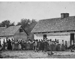
Slavery in the United States was an institution that had a large impact on the economic, political and social fabric of the country. The average price of a slave in 1860 was $800 and the economic magnitude of that price in today's values ranges from $17,000 to $266,000, depending on the index used.

In that year, there were an estimated four million slaves living in the South and it is estimated that their aggregate market value was over $3 billion then. That corresponds to $10 trillion today (as a share of GDP).

For a discussion of these issues, see Measuring Slavery in 2016 Dollars.

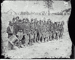
• The Civil War was one of the most devastating events in the history of the United States. It lasted from 1861 to 1865 and has been estimated to have a direct cost of about $6.7 billion valued in 1860 dollars. If this number were evaluated in dollars of today using the GDP deflator it would be $151 billion, less than one-fourth of the current Department of Defense budget. This would be inappropriate, as would be using the wage or income indexes. The only measure that makes sense for an expenditure of this size is to use the share of GDP, as the war impacted the output of the entire country. Thus the relative value of $6.7 billion of 1860 would be $28.35 trillion today, or over 170% of our current GDP.

  The $6.7 billion does not take into account that the war disrupted the economy and had an impact of lower production into the future. Some economic historians have estimated this additional, or indirect cost, to be another $7.3 billion measured in 1860 dollars. This means the cost of the war (as a share of the output of the economy) was nearly $59 trillion as measured in current dollars.

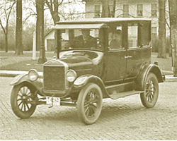
The Model T Ford cost $850 in 1908; however, by 1925 the price had fallen to $290. How do we compare these values? If you wanted to compare the two years you would see that by using the CPI, the GDP deflator or the consumer bundle, $850 in 1908 is equivalent to a value between $1,485 and $1,670 in 1925. Using the wage indicator we see that the labor cost (of the 1908 car in 1925 wages) was $2,094 and by using the GDP per capita indicator it was $1,957. Thus in 1925 the $290 was less than 20% of its cost in 1908 using the price indexes and only 11 to 14% using the wage indicators and 15% using the GDP per capita.

If we wanted to consider the costs of the Model T using today's prices we would find that the $850 cost in 1908 is $22,900 in today's prices using the CPI, $16,600 using the GDP deflator, about $52,500 using the consumer bundle, $98,600 using the unskilled wage, $166,600 using the manufacturing compensation, and $142,300 when comparing using the GDP per capita. At this point the Ford was a luxury for most everyone.

The $290 in 1925, on the other hand, would be only $3,970 in today's prices using the CPI, $3,200 using the GDP deflator, $8,800 using the consumer bundle, $13,700 using the unskilled wage, $18,400 using the manufacturing compensation, and $21,000 when comparing using the GDP per capita. By then, the ford was an automobile affordable by all.

Babe Ruth signed a contract on March 10, 1930 with the American League Base Ball Club of New York (The Yankees) to play baseball for the next two years at an annual salary of $80,000. In 2016, the CPI was 16 times larger than it was in 1931, and the GDP deflator was 13 times larger. This means that if we are interested in Ruth's purchasing power of housing or meals, then he was "earning" the equivalence of about $1,260,000 today.

In 2016, the average consumer unit spends about 32 times in dollars more than it spent 81 years earlier. Thus, if we want to compare Ruth's earnings using the index of what the average household buys, it would be over $2,975,000 today. The relative cost of labor is 46 times (unskilled) and 64 times (manufacturing production workers) higher in 2016 than in 1931. So if we wanted to compare his wage to what someone selling hot dogs would earn, we could say his "relative wage" is four to five million.

GDP per capita and GDP are 83 and 210 times larger in 2016 than they were in 1931. Thus, Ruth's earnings relative to the average output would be $7,400,000 today. Finally, as a share of GDP, Ruth's "output" that year would be $19,100,000 in today's money.

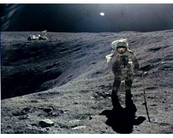
Putting a man on the moon: in March of 1966) NASA told Congress the "run-out cost" of the Apollo program (to put men on the moon) would be an estimated $22.718 billion for the 13 year program that accomplished six successful missions of putting astronauts on the moon between July 1969 and December 1972. (http://www.hq.nasa.gov/office/pao/History/SP-4009/keyev4.htm) According to Steve Garber, NASA History Web Curator, the final cost was between $20 and $25 billion.

How much would that be today? If we used the CPI, it would be $160 billion, but this would not be a very good measure since the CPI does not reflect the cost of rockets and launch pads. Using the consumer bundle would not be relevant either. Using the broader based GDP deflator gives a present cost of $132 billion. An alternative would be to use the production worker indicator as a rough measure of the labor cost in current terms and that would be $231 billion. By using the GDP per capita, we are measuring the cost in terms of average product and would get a number of $315 billion. Finally, a way to consider the "opportunity cost" to society, the best measure might be the cost as a percent of GDP, and that number would be $518 billion. This amount over thirteen years would be $40 billion per year. As a comparison, the NASA budget for the current fiscal year is approximately $19 billion.

The "real" price of gasoline: Gasoline cost 27 cents a gallon in 1949 compared to around $2.35 today.* How has the relative cost of buying gas changed over the last 63 years? Presented here are two tables computing the annual "real" cost using our seven indicators, one in 2016 dollars, and the other in 1949 dollars. While the two tables show the same trends, they do give a different perspective.

Using the 2016 table and the CPI and the GDP deflator, we see that gasoline was quite expensive in 2012 and it was the cheapest in 1998. Today, the real price using these two measures is higher than the decade ofthe 1990s.

By looking at the share of the Consumer Bundle and GDP per capita, the story is a bit different. In 1981, a gallon of gas took as much out of what the average consumer spent as $4.64 did in 2016. And as a share of GDP per capita, gas was even more expensive in those earlier days as it was over $5.57 in 1980 and as much as $8.48 in 1949.

The other table tells the story in a different way. Let us look at relative cost to a worker to fill up using 1949 dollars. That year the 27 cents it cost for a gallon of gas, took a certain share of the worker's wage. The interesting question is, has the cost as a share or percent of the worker's wage increased or decreased over time? The table shows that for the two wage rates and price of gasoline in other years, this cost has fallen. Since wages have increased faster than the price of gasoline, by 2016 an unskilled worker spends less than one-half as much, as a percent of wages, for a gallon of gasoline than the 1949 worker. For a production worker it is a little more than a third. The table shows that the $2.18 a worker paid in 2016 would be comparable to only 13 to 10 cents (in 1949 prices "share" of the wage.)

When we use the GDP per capita, the cost has fallen faster. Looking at the table shows that a gallon of gasoline today costs around 7 cents a gallon (in 1949 prices) if measured as a "share" of the GDP per capita. This is because in 1949, 27 cents was 0.015% of per capita GDP, while in 2016, $2.18 was 0.00012%.

Finally, comparing its cost as a share of GDP, we see that in 1949 prices, it is about 3 cents. This means that a gallon of gasoline was over eight times larger as a share of output in 1949 than it is today.

* The nominal price of gasoline can be found at found at: http://tonto.eia.doe.gov/dnav/pet/pet_pri_gnd_dcus_nus_a.htm
For the tables used here, I used the price of a gallon of leaded regular from 1949 to 1976, the average of the price of leaded regular and unleaded regular from 1977 to 1990 and the price of unleaded regular from 1991 to 2016.

Real Price is measured using the relative cost of a (fixed over time) bundle of goods and services such as food, shelter, clothing, etc., that an average household would buy. In theory the size of this bundle does not change over time, however, adjustments are made for the items in the bundle. This measure uses the CPI.

Real Value is measured using the relative cost of the amount of goods and services such as food, shelter, clothing, etc., that an average household would buy. Historically this bundle has become larger as households have bought more over time. This measure uses the Value of the Consumer Bundle, which is only available after 1900.

Labor Value is measured using the relative wage a worker would use to buy the commodity. This measure uses one of the wage indexes.

Income Value is measured using the relative average income that would be used to buy a commodity. This measure uses the GDP per capita.

Historic Standard of Living measures the purchasing power of an income or wealth in its relative ability to purchase a (fixed over time) bundle of goods and services such as food, shelter, clothing, etc., that an average household would buy. This bundle does not change over time. This measure uses the CPI.

Contemporary Standard of Living is measured using the relative cost of the amount of goods and services such as food, shelter, clothing, etc., that an average household would buy. This bundle has become larger over time as households have bought more over time. This measure uses the Value of the Consumer Bundle, which is only available after 1900.

Labor Earnings measures the amount of income or wealth relative to the wage of the average worker. This measure uses one of the wage indexes.

Economic Status measures the relative "prestige value" of an amount of income or wealth measured using per capita GDP. When compared to other incomes or wealth, it shows the relative prestige the owners of this income or wealth because of their rank in the income distribution. This measure uses GDP per capita.

Economic Power measures the amount of income or wealth relative to the total output of the economy. When compared to other incomes or wealth, it shows the relative "influence" of the owner of this income or wealth has in controlling the composition or total-amount of production in the economy. This measure uses the share of GDP.

Historic Opportunity Cost of a project is measured by comparing its relative cost using the cost index of all output in the economy. This measure uses the GDP Deflator.

Contemporary Opportunity Cost is the cost of a project relative to the amount the average household spends annually on consumer goods and services. The project may pertain either to business/government, a person/household, or to a nonprofit institution. This measure uses the Value of the Consumer Bundle, which is only available after 1900.

Labor Cost of a project is measured using the relative wage of the workers that might be used to build the project. This measure uses one of the wage indexes.

Economy Cost of a project is measured using the relative share of the project as a percent of the output of the economy. This measure indicates the opportunity cost in terms of the total output of the economy. The viewpoint is the importance of the item to society as a whole, and the measure is the most inclusive. This measure uses the share of GDP.

The CPI is most often used to make comparisons partly because it is the series with which people are most familiar. This series tries to compare the cost of things the average household buys such as food, housing, transportation, medical services, etc. For earlier years, it is the most useful series for comparing the cost of consumer goods and services. It can be interpreted as how much money you would need today to buy an item in the year in question if its price had changed the same percentage as the average price change.

• Construction of CPI Indicator

The GDP Deflator is similar to the CPI in that it is a measure of average prices. The "bundle" of goods and services here includes all things produced in the economy, not just consumer goods and services that are reflected in the CPI.

• Construction of GDP Indicator

The Consumer Bundle is the average dollar value of the annual expenditures of a "consumer unit." The consumer unit could be a family or another type of household. The main point is that spending is a joint decision of the members of the unit. The bundle increases over time as household income increases. Unlike the CPI, not only the cost, but also the amount of goods and services increases over time.

• Construction of the Consumer Bundle Indicator

The Unskilled Wage is a good way to determine the relative cost of something in terms of the amount of work of unskilled labor that it would take to produce, or the relative time spent at work by unskilled workers in order to earn its cost. This indicator can also be useful in comparing different wages over time. The unskilled wage is a more consistent measure than the average wage for making comparisons over time. This is because the average wage changes both because of changes in the composition of skills in the workforce as well as the general cost of labor. The level of skills of the unskilled is assumed to stay the same.

• Construction of Unskilled Wage Indicator

Compensation of Production Workers is an alternative way to determine the relative cost of something in terms of the amount of work by a specific group of workers. In this case it is manufacturing production workers, which would include blue-collar workers, hourly rated workers, or non-office workers. Unlike the unskilled wage, this series includes both money earnings and benefits. During the last third of the 20th century, benefits grew to be close to 25% of the compensation.

• Construction of the Compensation of Production Workers

The GDP per capita is an index of the economy's average output per person and is closely correlated with the average income. It can be useful in comparing different incomes over time.

• Construction of GDP Indicator

The GDP is the market value of all goods and services produced in a year. Comparing an expenditure using this measure tells you how much money in the comparable year would be the same percent of all output.

• Construction of GDP Indicator